Last week, we discussed some of the difficulties involved in reconstructing the landscape of the First Cataract region, focusing in particular on how we can use satellite imagery, historical maps, and aerial photography in tandem with archaeological finds to get a better idea of how this landscape might have looked in antiquity. In the coming weeks, we will take a more general look at the basic kinds of spatial analysis we will be performing, and the kinds of questions such analyses may hope to answer. However, to lay the groundwork for this discussion, I want to focus this week on one of the most important components that we need in order to perform many kinds of spatial analysis.
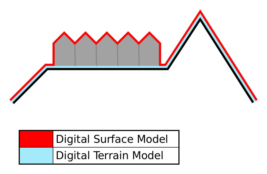
This is the humble Digital Elevation Model (DEM), sometimes also referred to as a Digital Terrain Model (DTM) or Digital Surface Model (DSM). You can think of a DEM as a model of the earth’s surface. Generally speaking, Digital Terrain Models show a bare topographic representation of the earth’s elevation, while Digital Surface Models include objects on the earth’s surface like buildings, houses, and trees as well. Digital Elevation Model is not as specifically defined—some of the literature prefers to use the term DEM as an equivalent of DTM or DSM, though many now use DEM as a kind of generic term that may encompass both.
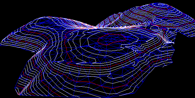
Digital elevation models are generally represented in one of two different formats: as a raster image, or as a vector based network. The difference between such models is relatively simple, in a raster image, each individual pixel is assigned an elevation value. This value is typically computed from pre-existing topographic data. Now of course, the resolution of each image may vary, sometimes dramatically. Freely available data often has a resolution of 30m or even less—thus each pixel represents a 30 x 30 m square of terrain. Commercial DEMs are often much, much finer—with resolutions as detailed as 1 m! The more precise the DEM, the more fine-grained conclusions one can offer! Raster-based DEMs are sometimes referred to as secondary, or computed DEMs, since they infer an elevation value for an entire pixel from individual readings at specific points. In contrast, a vector based network relies on geometric lines to represent a continuous 3D surface. This network is usually comprised of a three dimensional mesh of irregular triangles, and is often abbreviated as a TIN (Triangulated Irregular Network).
Vector models are sometimes referred to as measured DEMs, since they rely on particularly intensive topographic mapping procedures that directly measure the elevation of an entire surface. They are often used at the site level, or even to represent individual objects, but without massive amounts of computing power and topographic readings, they are often less feasible for representing large areas. Given that the Borderscape Project covers over 10,000 km2, our project relies primarily on raster based elevation models. Generally speaking, when one sees the term DEM in scholarly literature, it is reasonable to assume that this implies a raster image unless otherwise stated.
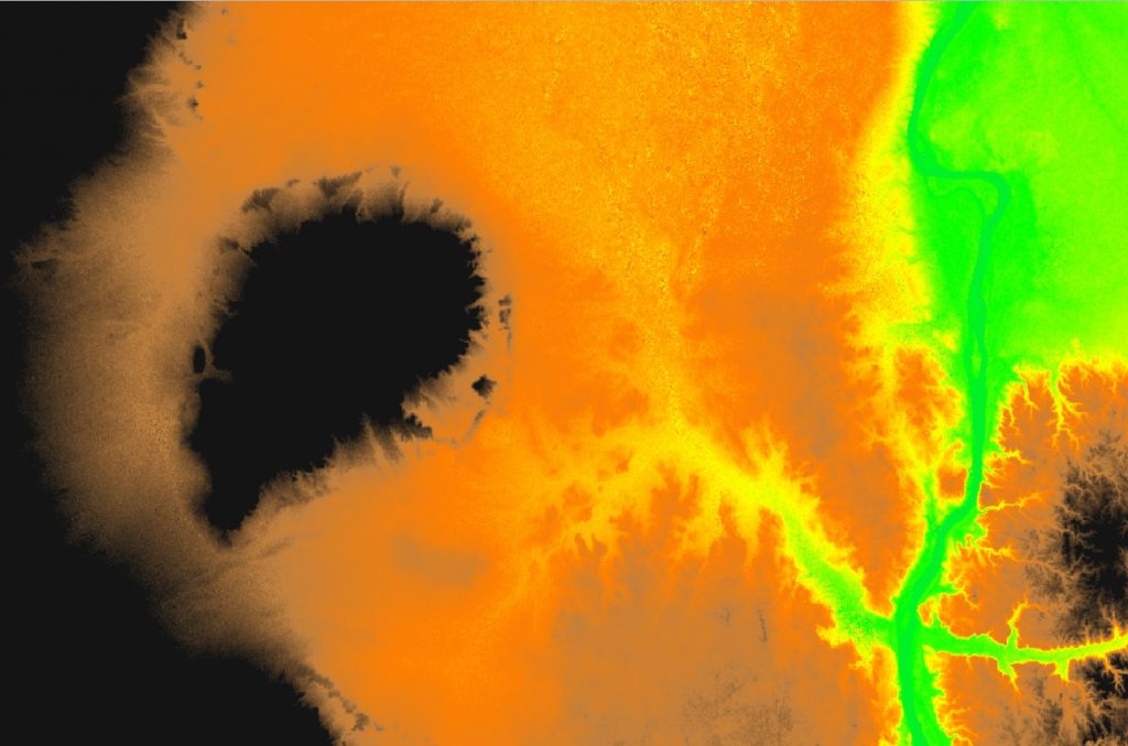
Often, it is necessary to introduce a color ramp to allow features within a DEM to “pop” more easily for the human eye. For example, in the image of our study area below, we can see how green represents the lowest altitudes, while yellows, reds, and especially darker brown and black represent higher altitudes.
A digital elevation model is a prerequisite for many different kinds of spatial analysis, some of which we will discuss in the coming weeks, from flood modelling to viewsheds. It is one of the most important tools available for archaeological projects hoping to use GIS to perform any kind of wider, regional analyses. Thankfully, relatively high quality DEMs are freely available from the US Geological Society’s Earth Explorer module. The Shuttle Radar Topography Mission’s data is a phenomenal resource that provides essentially global coverage, allowing scholars to download tiles of relevant data for their particular study area.
However, it is worth noting that the kinds of spatial analysis that should be performed are always contingent upon one’s research questions. For the Borderscape Project, there are three primary research foci: 1) What did the ancient landscape look like (discussed briefly last week)? 2) How was this landscape used, and how did this change over time? 3) How does the social landscape correspond to patterns of land use, settlement, and natural resources? All of our spatial analyses are geared towards answering aspects of these three important questions. Next week, we will take a more detailed look at various types of spatial analysis where we can combine a DEM with historical data and archaeological evidence to infer patterns of landscape use.